S0 — Sensor & Calibration Models

The mathematical foundation upon which the entire pipeline is built. S0 is not an algorithmic step — it is the collection of physical and geometric measurement functions that map the 3D continuous world into the discrete pixels and inertial samples the filter consumes. Every residual, state propagation step, and EKF update Jacobian in the system is built on top of S0.

A bug in S0 (such as a coordinate system flip or a sign error in the Jacobian) does not fail loudly with an exception. Instead, it quietly poisons every downstream stage, manifesting as mysterious, untraceable quadratic drift or immediate filter divergence.

---

1. Camera Projection Models

A camera model defines the mapping:

$$\text{project}(\mathbf{p}_c) \rightarrow \mathbf{z} = [u, v]^T$$

where $\mathbf{p}_c = [x, y, z]^T \in \mathbb{R}^3$ is a 3D point in the camera-frame coordinate system. Cortex supports both the standard Pinhole-RadTan model (for rectilinear lenses) and the Kannala-Brandt model (for wide-angle fisheye lenses).

A. Pinhole Projection (The Core Perspective)

The ideal pinhole camera projects the 3D camera-frame coordinate $\mathbf{p}_c$ to the normalized image plane coordinates $\mathbf{x}_n = [x_n, y_n]^T$:

$$x_n = \cfrac{x}{z}, \qquad y_n = \cfrac{y}{z}$$

These are then mapped to pixel coordinates via focal lengths ($f_x, f_y$) and principal points ($c_x, c_y$):

$$u = f_x x_n + c_x, \qquad v = f_y y_n + c_y$$

Understanding the Model Parameters:

• Focal Lengths ($f_x, f_y$): Represent the distance between the lens optical center and the image sensor plane, expressed in pixel units. These scale the normalized coordinates to match the physical pixel spacing on the silicon wafer.
• Principal Points ($c_x, c_y$): Represent the exact pixel coordinate where the camera’s optical axis physically pierces the image sensor. Because the lens assembly is never perfectly centered on the silicon during manufacturing, the principal point is almost never exactly at the geometric center of the pixel grid.

B. Distortion Models (Modeling Lens Curvature)

Real lenses bend light, introducing distortion. Before mapping to pixels, the normalized coordinates $\mathbf{x}_n$ are warped to distorted coordinates $\mathbf{x}_d = [x_d, y_d]^T$.

1. Radial-Tangential (RadTan) Distortion (5-Lens / 4-Intrinsic Parameters)

The complete camera projection model combines 5 lens distortion parameters ($k_1, k_2, k_3, p_1, p_2$) and 4 intrinsic calibration parameters ($f_x, f_y, c_x, c_y$):

• Radial Distortion ($k_1, k_2, k_3$): Models barrel/pincushion lens symmetry. Glass lenses curve more aggressively near their outer borders. This pulls or pushes pixels along radial lines emerging from the optical center: $$r^2 = x_n^2 + y_n^2$$ $$\text{radial\_correction} = 1 + k_1 r^2 + k_2 r^4 + k_3 r^6$$
• Tangential Distortion ($p_1, p_2$): Models “decentering” or “thin prism” distortion. This is caused by individual lens elements being slightly tilted relative to each other or misaligned relative to the image sensor plane during assembly, creating a slight physical warp:

$$x_d = x_n \cdot \text{radial\_correction} + 2 p_1 x_n y_n + p_2 (r^2 + 2 x_n^2)$$ $$y_d = y_n \cdot \text{radial\_correction} + p_1 (r^2 + 2 y_n^2) + 2 p_2 x_n y_n$$

2. Kannala-Brandt (KB) Fisheye Distortion (4-Parameters)

Wide-angle fisheye lenses cannot be modeled by simple rectilinear perspective because their field of view often exceeds $180^\circ$ (light rays can literally bend around behind the camera origin).

Instead of assuming light travels in straight lines to a flat plane, the Kannala-Brandt model maps the angular direction of the incoming light ray ($\theta$) relative to the optical axis using an odd-power polynomial series:

$$r = \sqrt{x_n^2 + y_n^2}, \qquad \theta = \text{atan2}(r, 1)$$ $$d(\theta) = \theta + k_1 \theta^3 + k_2 \theta^5 + k_3 \theta^7 + k_4 \theta^9$$

The distorted coordinates are then mapped:

$$x_d = \cfrac{d(\theta)}{r} x_n, \qquad y_d = \cfrac{d(\theta)}{r} y_n$$

• Optical Center Limit (r = 0): When $r = 0$ (the principal ray), the angle $\theta = 0$, and the ratio $d(\theta) / r$ is mathematically defined as its limit: $\lim_{r\to0} d(\theta)/r = 1$. Thus, at the principal point, $x_d = x_n = 0$ and $y_d = y_n = 0$ with zero distortion, preventing any division-by-zero NaN values.

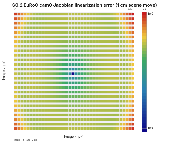
C. The Analytical Projection Jacobian

To perform the EKF Measurement Update (where we update our state estimate using the visual tracking error), we need to write the derivative of pixel coordinates $\mathbf{z} = [u, v]^T$ w.r.t the 3D camera-frame point $\mathbf{p}_c$. This Jacobian, $\mathbf{H}_p$, is computed via the chain rule:

$$\mathbf{H}_p = \cfrac{\partial \mathbf{z}}{\partial \mathbf{p}_c} = \cfrac{\partial \mathbf{z}}{\partial \mathbf{x}_d} \ccdot \cfrac{\partial \mathbf{x}_d}{\partial \mathbf{x}_n} \ccdot \cfrac{\partial \mathbf{x}_n}{\partial \mathbf{p}_c}$$

• Pinhole Quotient Rule: The normalized image coordinate is a quotient of coordinates: $x_n = x/z$. Under the standard quotient rule, its derivatives w.r.t the 3D coordinate vector $\mathbf{p}_c = [x, y, z]^T$ are given by:
  • $\partial x_n/\partial x = 1/z
  • $\partial x_n/\partial y = 0
  • $\partial x_n/\partial z = -x / z^2 This forms the linear perspective term:

$$\cfrac{\partial \mathbf{x}_n}{\partial \mathbf{p}_c} = \begin{bmatrix} 1/z & 0 & -x/z^2 \ 0 & 1/z & -y/z^2 \end{bmatrix}$$

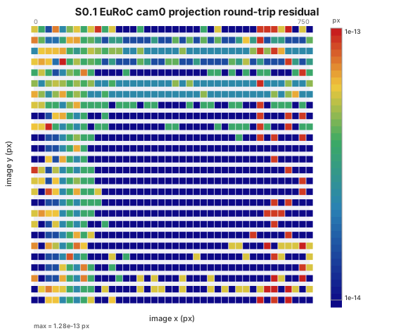
Cortex checks the rank of $\mathbf{H}_p$ (which must be strictly 2) and validates its analytic derivatives against numerical finite differences during unit testing down to machine precision ($\approx10^{-15}$).

---

2. Inertial Sensor (IMU) Physics

An Inertial Measurement Unit (IMU) consists of a 3-axis gyroscope and a 3-axis accelerometer. The continuous-time physical models are:

$$\tilde{\boldsymbol{\omega}}(t) = \boldsymbol{\omega}(t) + \mathbf{b}_g(t) + \mathbf{n}_g(t)$$ $$\tilde{\mathbf{a}}(t) = \mathbf{R}_{W}^{I}(t) \left( \mathbf{a}_W(t) - \mathbf{g}_W \right) + \mathbf{b}_a(t) + \mathbf{n}_a(t)$$

Where:

• $\tilde{\boldsymbol{\omega}}, \tilde{\mathbf{a}}$: The raw gyro and accelerometer measurements.
• $\boldsymbol{\omega}, \mathbf{a}_W$: The true angular velocity and true world-frame acceleration of the IMU.
• $\mathbf{b}_g, \mathbf{b}_a$: The slow-varying sensor biases (modeled as random walks).
• $\mathbf{n}_g, \mathbf{n}_a$: White Gaussian measurement noise.
• $\mathbf{g}_W$: The global gravity vector.

Why an IMU Resting on a Table Reads $+9.81\text{ m/s}^2$

This is a common point of confusion for beginners. Accelerometers measure specific force (the reaction force relative to free-fall), not true acceleration. When an IMU is stationary on a flat table:

• Its true world acceleration is $\mathbf{a}_W = \mathbf{0}$.
• The world gravity is $\mathbf{g}_W = [0, 0, -9.81]^T$.
• Thus, the accelerometer reads:

$$\tilde{\mathbf{a}} = \mathbf{R}_W^I (\mathbf{0} - [0, 0, -9.81]^T) = \mathbf{R}_W^I [0, 0, 9.81]^T$$

• This registers as a $+9.81\text{ m/s}^2$ upward acceleration. A VIO pipeline must subtract gravity during propagation to prevent the drone from quadratically shooting off into the sky in its state estimate.

---

3. Space-Time Calibration

Sensors do not live at the same physical point, nor do they capture data at the exact same instant. We must calibrate both spatial and temporal offsets.

A. Spatial Extrinsics (6-DoF Calibration)

The camera is offset from the IMU center by a translation $\mathbf{p}_{ic}$ and a rotation $\mathbf{R}_{ic}$ (or $\mathbf{T}_{ci} \in \text{SE}(3)$). A point $\mathbf{p}_f$ in the world frame is mapped to the camera frame $C$ via the intermediate IMU frame $I$:

$$\mathbf{p}_{\text{imu}} = \mathbf{R}_{W}^{I} (\mathbf{p}_f - \mathbf{p}_{\text{W\_imu}})$$ $$\mathbf{p}_{\text{cam}} = \mathbf{R}_{\text{ic}}^T (\mathbf{p}_{\text{imu}} - \mathbf{p}_{\text{ic}})$$

Under dynamic motion, omitting even a $1\text{ cm}$ offset introduces massive unmodeled centripetal and Euler accelerations into the camera’s visual track:

$$\mathbf{a}_{\text{cam}} = \mathbf{a}_{\text{imu}} + \mathbf{\omega} \times (\mathbf{\omega} \times \mathbf{p}_{\text{ic}}) + \cdot{\mathbf{\omega}} \times \mathbf{p}_{\text{ic}}$$

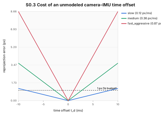
B. Temporal Extrinsics (Time-Offset Calibration)

Due to transmission latency, clock drift, or rolling shutters, there is a time delay $t_d$ between the camera clock and the IMU clock:

$$t_{\text{camera}} = t_{\text{imu}} - t_d$$

If the drone is rotating at a moderate angular velocity of $100^\circ\text{/s}$ (common in maneuvers), a tiny $5\text{ millisecond}$ unmodeled time offset ($t_d = 0.005$) introduces a $0.5^\circ$ alignment error. This is equivalent to several pixels of visual tracking error, causing the EKF update to inject false corrections.

---

The S0 Contract

The contract defines the required behavior of the sensor and calibration mathematical block:

Element	Contract Specification
Signature	$\text{project}(p_c, \zeta) \rightarrow (u,v)$
Pre-conditions	Focal lengths $f_x, f_y > 0$; distortion parameters are within stable convergence bounds; gravity vector orientation is frame-consistent.
Post-conditions & Invariants	1. Round-Trip consistency: $\text{unproject}(\text{project}(p_c)) \approx p_c / \|p_c\|$ down to $10^{-15}$ machine precision for all depth $z > 0$. 2. Jacobian rank: Projection Jacobian $\mathbf{H}_p$ is strictly rank-2 and matches numerical finite-differences. 3. Cheirality: Points behind the lens ($z \le 0$) are rejected, never projected. 4. Inertial Identity: A zero-noise, gravity-compensated stationary IMU integrates to exactly zero velocity and zero translation over time.

---

Real-Data Validation via s0_inspect

Cortex provides a generalized static release tool, s0_inspect, which can be invoked directly on actual EuRoC sensor streams to verify physical calibration.

# Execute the real-data sensor inspector on EuRoC V1_01_easy
s0_inspect --dataset /path/to/V1_01_easy/mav0 --out build/s0 --frame 0

This generates two critical diagnostic overlays:

A. Camera Model Overlay (distortion.svg)

Superimposes an ideal, distortion-free rectilinear grid (grey) against the actual lens-warped grid (green) calculated from the distortion coefficients. It draws lens displacement vectors and verifies the round-trip projection error across every node of the grid. This allows you to visually inspect and confirm that the lens model is perfectly inverting the camera’s physical barrel distortion.

B. IMU Allan Deviation Curve (imu_allan.svg)

Computes the Allan Deviation of the gyroscope and accelerometer streams under static conditions. The Allan deviation curve (plotted on a log-log scale) allows you to extract:

1. White Noise Density (N): Sourced from the slope of $-0.5$ at $t = 1\text{ s}$. This represents the continuous-time noise parameters used in the process noise covariance $\mathbf{Q}$.
2. Bias Instability (B): Sourced from the flat bottom of the curve.
3. Random Walk (K): Sourced from the slope of $+0.5$ at long integration times.

Running s0_inspect on the physical drone rig allows you to verify that your configured process noises exactly match the true physical noise profile of the sensor, protecting the filter from initial over-confidence.