The VIO Pipeline Overview

Visual-Inertial Odometry (VIO) fuses a camera (rich geometry, slow, scale-ambiguous if monocular) and an IMU (fast, senses gravity, drifts quadratically when integrated alone) into a single, high-rate metric estimate of where the platform is — and, just as importantly, how uncertain that estimate is.

Despite its elegance, VIO is notoriously difficult to implement. In practice, Kalman filtering is extremely sensitive to minor misalignments, sensor configurations, and timing offsets. A single 1-pixel projection error or a minor sign flip in a Jacobian can cause the filter’s reported uncertainty to collapse, understating its true error. This is the dreaded over-confidence bug where the filter claims absolute certainty while silently drifting away.

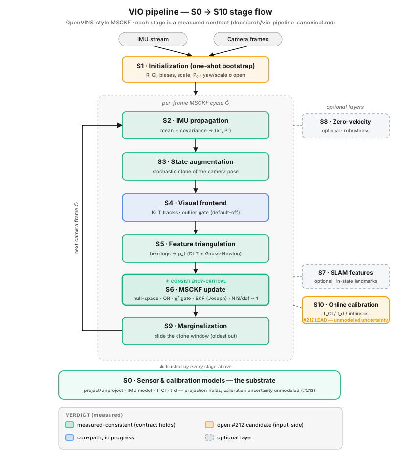
This section documents the VIO pipeline cortex implements, stage by stage. To isolate and conquer the bugs that plague VIO development, each stage is treated as a rigorous mathematical contract: specifying its why, what, and how, its pre-conditions, its post-conditions, and the diagnostics/unit probes used to prove its consistency.

The Core Challenge: Fusing Two Worlds

To understand why VIO is so sensitive, we must look at the physical nature of the two sensors we are trying to bind:

Metric	Camera (Visual)	IMU (Inertial)
Observation Type	High-dimensional pixel arrays (photometric).	Acceleration ( $\mathbf{a}$ ) and angular velocity ( $\boldsymbol{\omega}$ ).
Measurement Rate	Low rate (usually $10 - 30\text{ Hz}$ ).	High rate (usually $200 - 1000\text{ Hz}$ ).
Drift Profile	Drift-free under static conditions, but scale-ambiguous in monocular setups.	Quadratic drift in position ( $t^2$ ) and linear drift in velocity ( $t$ ) over time.
Observability	Excellent for relative rotation and bearing directions; cannot observe absolute scale from a single camera.	Directly observes absolute roll, pitch (via gravity direction), and physical scale (via acceleration).

Without the IMU, a monocular camera cannot tell the difference between moving $1\text{ meter}$ in a small room or $100\text{ meters}$ in a giant canyon. Without the camera, the IMU’s double-integration of raw accelerometer noise would drift by kilometers in minutes. Fusing them requires absolute mathematical synchrony.

The Coordinate Frame Glass House

The most common failure mode in VIO engineering is coordinate frame misalignment. A VIO pipeline is a “mathematical glass house”—if any of the coordinate relationships are defined inconsistently, the entire estimator collapses quadratically.

Our coordinate frame relationships are mapped in the following diagram:

VIO Coordinate Frames Map: Showing the spatial transformations from World frame (gravity-aligned) to IMU/Body frame, and from IMU frame to Camera frame via rigid extrinsics R_ic and p_ic.

Cortex enforces a rigid, unified convention across all eleven stages:

World Frame ( $W$ ): The global reference frame. Gravity is aligned with the global z-axis: $\mathbf{g}_W = [0, 0, -9.81]^T$ . Yaw (heading) and global position are unobservable in this frame.
IMU Frame ( $I$ ): The body frame of the vehicle. Raw acceleration $\mathbf{a}_{\text{imu}}$ and angular rate $\boldsymbol{\omega}_{\text{imu}}$ are sensed relative to this frame.
Camera Frame ( $C$ ): The camera coordinate system. The optical axis points along the positive z-axis ( $+z$ is forward/depth).
Extrinsics ( $\mathbf{R}_{\text{ic}}$ , $\mathbf{p}_{\text{ic}}$ ): The rigid 6-DoF transform mapping the IMU body center to the Camera origin (IMU-to-Camera extrinsics):

\mathbf{p}_{\text{cam}} = \mathbf{p}_{\text{imu}} + \mathbf{R}_{\text{wi}} \mathbf{p}_{\text{ic}}

\mathbf{R}_{\text{wc}} = \mathbf{R}_{\text{wi}} \mathbf{R}_{\text{ic}}

Clones: The Core MSCKF State

In visual-inertial odometry, the concept of clones is instrumental to the algorithm and represents a first-order architectural block.

Instead of tracking 3D landmarks (features) directly in our EKF state vector—which would cause our covariance matrix to grow quadratically with the map size—the Multi-State Constraint Kalman Filter (MSCKF) tracks a sliding window of historic IMU poses, called clones.

When a camera frame is captured:

We “clone” the current IMU pose (orientation and position) into the EKF state covariance.
The visual frontend tracks landmarks across these clones.
When a landmark is lost or its track ends, we perform triangulation to estimate its 3D coordinate in the world.
We write a measurement Jacobian relating the landmark’s pixel observations to the cloned poses in our sliding window:

\mathbf{r} \approx \mathbf{H}_x \tilde{\mathbf{x}} + \mathbf{H}_f \tilde{\mathbf{p}}_f + \mathbf{v}

By projecting this Jacobian onto its left null space (multiplying by a matrix $\mathbf{V}^T$ such that $\mathbf{V}^T \mathbf{H}_f = \0$ ), we marginalize the landmark completely out of the EKF update:

\mathbf{V}^T \mathbf{r} \approx \mathbf{V}^T \mathbf{H}_x \tilde{\mathbf{x}} + \mathbf{V}^T \mathbf{v}

The landmark position $\tilde{\mathbf{p}}_f$ is completely eliminated from the EKF update! The EKF then corrects the cloned IMU poses directly through cross-covariance.

Hardware Compute Fabrics: Serial MCUs vs. Parallel KPUs

The decision to use MSCKF (which throws away landmarks) rather than SLAM (which retains landmarks in the state) is a computational trade-off driven by hardware:

Standard Serial MCUs (CPUs): Standard microcontrollers process instructions sequentially. Performing EKF updates on large matrices scales with cubic complexity ( $\mathcal{O}(N^3)$ where $N$ is state dimension). Keeping the matrix small by marginalizing landmarks (MSCKF) is essential to stay within the real-time loop.
Highly Concurrent Matrix-Oriented KPUs: Modern Embodied AI hardware introduces KPUs (Knowledge Processing Units / Tensor Cores). These are highly concurrent compute fabrics designed specifically for parallel, high-throughput matrix-multiplication operations (BLAS/LAPACK GEMM).
The SLAM Trade-off: If we have KPU hardware capable of processing large-scale matrices in parallel, retaining landmark states in the covariance matrix becomes highly desirable. While it grows the covariance matrix, keeping the landmarks allows the filter to preserve the exact spatial correlations, perform loop closures, and achieve significantly higher accuracy and robustness.

The Eleven Staged Contracts (S0–S10)

To isolate bugs, Cortex slices the MSCKF pipeline into eleven distinct, self-contained stages. Each stage is governed by a strict contract of pre-conditions and post-conditions:

Stage	Contract Page	Responsibility	Core Invariant / Math
S0	Sensor Models	Intrinsics & Extrinsics	Projects 3D points to 2D pixels; enforces distortion models (Radial, Equidistant).
S1	Initialization	State Seeding	Solves gravity alignment, gyro biases, and scale prior to launching the filter.
S2	IMU Propagation	EKF Predict Step	Propagates state mean and covariance forward using the exact 3rd-order discrete transition matrix.
S3	Pose Augmentation	State Cloning	Appends the current IMU pose to the covariance, maintaining exact Left-Invariant clones.
S4	Visual Frontend	Track Management	Detects corners, tracks them via KLT optical flow, and purges outliers via 2-point/5-point RANSAC.
S5	Triangulation	Structure Recovery	Reconstructs 3D coordinates of a feature track from multi-view bearings using least-squares.
S6	MSCKF Update	EKF Measurement Update	Performs Left Null-Space projection, QR compression, $\chi^2$ gating, and EKF state correction.
S7	SLAM Features	Persistent Landmarks	Integrates permanent 3D landmarks in the EKF state for long-term drift-free mapping.
S8	Zero-Velocity (ZUPT)	Stationary Robustness	Applies zero-velocity pseudo-measurements to constrain drift when the drone is stationary.
S9	Marginalization	Window Pruning	Drops the oldest clone, correctly transferring its cross-covariance block out of the window.
S10	Online Calibration	Self-Correction	Estimates 6-DoF IMU-to-Camera extrinsics and time-offsets online within the filter state.

What “Good” Looks Like: Accuracy vs. Consistency

In visual-inertial odometry, accuracy is not enough. You can have sub-meter drift but still have a borked filter that crashes your drone. A healthy VIO pipeline must satisfy two distinct properties:

1. Accuracy (The Metric Drift)

Measured using Absolute Trajectory Error (ATE) and Relative Pose Error (RPE). Proves that your integration, camera projection, and triangulation are geometrically aligned.

2. Consistency (The Safety Property)

Consistency means the filter is honest. When the covariance matrix $\mathbf{P}$ claims the drone’s position is known to $\pm10\text{ cm}$ , the true position error must indeed be roughly within that $\pm10\text{ cm}$ envelope.

Over-Confidence: If the error is $1.5 \text{ m}$ but the covariance claims $\pm5\text{ cm}$ , the filter is over-confident. The state estimator will discard new visual measurements because it “thinks” it knows its position perfectly, causing the filter to diverge completely under aggressive motion.
Consistency is verified mathematically using the Normalized Innovation Squared (NIS) and Normalized Estimation Error Squared (NEES) metrics. For an $N$ -DoF state estimator, the expectation of raw NEES is $N$ :

E[\epsilon_{\text{NEES}}] = N

Often, we divide by $N$ to get Normalized NEES (the form reported on our diagnostics and sweeps), whose theoretical expectation is $1$ :

E\left[\cfrac{\epsilon_{\text{NEES}}}{N}\right] = 1

When Normalized NEES is close to 1, the filter is consistent. If it is significantly larger than 1, the filter is over-confident.

Exploring the Pipeline

Dive into the individual stages using the sidebar navigation, or learn about our diagnostic methodology and how we measure consistency:

Read Reading the metrics to understand NIS, NEES, and chi-squared testing.
Explore the Diagnostic Methodology to see how we isolate stage-level bugs.
Check out the Engineering Status page to see the latest consistency sweeps across the EuRoC MAV datasets.